V3: Simulation using 2-stage random effects
Relating two-stage random effects to simulated data and model output
Introduction
This chapter accompanies the 3rd video in the series, “Simulating data using the 2-stage random effects formulation”. The purpose of this chapter is to help in understanding the two-stage random effects formulation for mixed models by simulating data based on the formulation, analyzing the simulated data and comparing the two. This is a great way to wrap your head around what a mixed model is doing. This is written under the assumption that you have seen the first few videos in the Mixed Models series on the MumfordBrainStats YouTube channel. If you haven’t, go look for that playlist and watch those first. As discussed in the videos, this is not a perfect setup for the mixed models and not all mixed models can fit into this formulation, but it is a great way to understand mixed models. Sometimes it is helpful to see how repeated measures data are simulated in order to understand what the model is doing. In this case the values in the simulation will show up again when the data are fit using the lmer() function. Make sure to spend time matching up the values in the simulation code with the lmer output to increase your understanding of mixed models.
Data simulation
The simulation follows the two-stage random effects formulation in reverse to make up some fake data that look similar to the Sleepstudy data. Typically simulations are used for estimating type I error and power, but they are great for learning too. The benefit in simulation is the truth is known and be compared with the estimates. Specifically,the true group intercept and slope as well as all of the variance parameters will be known in this case.
Review of the two-stage formulation
Reviewing the two-stage formulation, recall the first stage of the model is \[Y_i = Z_i\beta_i + \epsilon_i, \: \epsilon_i\sim N(0, \sigma^2I_{n_i})\] and the second stage is \[\beta_i = A_i \beta + b_i, \: b_i \sim N(0,G).\] In these early examples \(A_i\) is an indentity matrix, so you can ignore it. This is because we’re only averaging within-subject effects in these models. In this case \(Y_i\) contains the average reaction times for subject \(i\) over 10 days, \(Z_i\) is the design matrix with a column of 1s and a column for days (0-9), \(\beta_i\) is the vector with the slope and intercept for subject \(i\) and \(\sigma\) is the within-subject variance. Notably, this variance is assumed to be the same for all subjects, as it does not have an \(i\) subscript. Last, \(n_i\), the number of observations for subject \(i\), is assumed to be 10 for all subjects, so \(I_{n_i}\) is a \(n_i\times n_i\) identity matrix. Here’s an example using the first subject in the data set (\(i\) would be 1),
\[\left[\begin{array}{c} 265 \\ 252 \\ 451 \\ 335 \\ 376 \\370 \\ 357 \\ 514 \\ 350 \\ 500 \end{array}\right] = \left[\begin{array}{cc} 1 & 0 \\ 1 & 1 \\ 1 & 2 \\ 1 & 3 \\ 1 & 4 \\ 1 & 5 \\ 1 & 6 \\ 1& 7 \\ 1 & 8 \\ 1 & 9 \end{array}\right]\left[\begin{array}{c} \beta_{0, i} \\ \beta_{1, i} \end{array}\right] + \left[\begin{array}{c} \epsilon_1 \\ \epsilon_2 \\ \epsilon_3 \\ \epsilon_4 \\ \epsilon_5 \\ \epsilon_6 \\ \epsilon_7 \\ \epsilon_8 \\ \epsilon_9 \\ \epsilon_{10} \end{array}\right].\]
The second level is looks like: \[\left[\begin{array}{c}\beta_{0,i} \\ \beta_{1,i}\end{array}\right] =\left[\begin{array}{c}\beta_{0} \\ \beta_{1}\end{array}\right] + \left[\begin{array}{c}b_{0,i} \\ b_{1,i}\end{array}\right],\] since the interest is in the average intercept and slope across subjects.
Data simulation based on two-stage formulation
To simulate the data, one goes through the two stages backwards, starting with stage 2. This setting assumes the random slope and intercept are independent, the intercept’s between-subject variance is \(24^2\) and slope’s between-subject variance is \(10^2\), so \[G=\left[\begin{array}{cc} 24^2 & 0 \\ 0 & 10^2 \end{array}\right].\] Another way to think of this, since the slope and intercept are independent is: \(b_{0,i}\sim N(0, 24^2)\) and \(b_{1,i}\sim N(0, 10^2)\). The true group intercept and slope are assumed to be 251 and 10, respectively, so subject-specific slopes and intercepts are generated using the multivariate normal distribution \[N\left(\left[\begin{array}{c} 251 \\ 10 \end{array}\right], \left[\begin{array}{cc} 24^2 & 0 \\ 0 & 10^2 \end{array}\right]\right).\]
It may not always be the case that the slope and intercept are independent. For example, sometimes the steepness of the slope may depend upon on where the subject started (the intercept). If they are very slow on the task on day 0, they may not decline as much over the following days compared to a person who starts off really fast. In this case, the off-diagonal of \(G\) would have a negative covariance value. In the interest of simplicity the independence assumption is used here, but the model fit will default to assuming they are correlated, which is fine. More on this to come.
To obtain the individual reaction times, the first stage is used based on the individual slope and intercept values that were generated with the multivariate Normal distribution above. Basically noise is added to that subject’s true regression line, with a variance of \(30^2\) to yield the subject-specific reaction times. The simulated data are then complete and ready for analysis.
Read through the function and pay attention to where the betas, G and sigma are. Relate them to the equations above and later find their estimates in the lmer output! I’ve flagged the numbers to take note of with comments.
library(ggplot2)
library(lme4)
library(lmerTest)
library(MASS)

makeFakeSleepstudyData = function(nsub){
  time = 0:9
  rt = c() # This will be filled in via the loop
  time.all = rep(time, nsub)
  subid.all = as.factor(rep(1:nsub, each = length(time)))

  # Step 1:  Generate the beta_i's.
  G = matrix(c(24^2, 0, 0, 10^2), nrow = 2)   ##!!! <- REMEMBER THESE NUMBERS!!!!
  int.mean = 251  ##!!! <- REMEMBER THESE NUMBERS TOO!!!!
  slope.mean = 10  ##!!! <- REMEMBER THESE NUMBERS TOO!!!!
  sub.ints.slopes = mvrnorm(nsub, c(int.mean, slope.mean), G)
  sub.ints = sub.ints.slopes[,1]
  time.slopes = sub.ints.slopes[,2]

  # Step 2:  Use the intercepts and slopes to generate RT data
  sigma = 30      ##!!! <- THIS IS THE LAST NUMBER TO REMEMBER!!!! (sorry for yelling)
  for (i in 1:nsub){
    rt.vec = sub.ints[i] + time.slopes[i]*time + rnorm(length(time), sd = sigma)
    rt = c(rt, rt.vec)
  }

  dat = data.frame(rt, time.all, subid.all)
  return(dat)
}
Generate and plot data
The following generates data for 16 subjects and plots them. This should look somewhat like the real sleepstudy data that were discussed in an earlier video.
set.seed(10) # this ensures you get what I got here
dat = makeFakeSleepstudyData(16)
ggplot(data = dat, aes(x = time.all, y = rt)) +
  geom_line() +
  geom_point() +
  facet_wrap(~subid.all)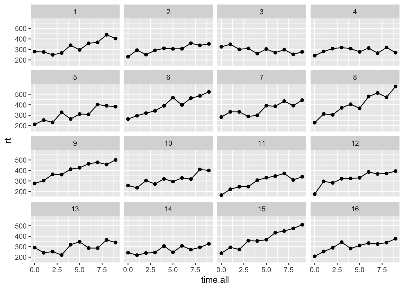
Run model and compare to simulation settings
Below is the appropriate model, which includes a random slope an intercept as well as a correlation between the two. To compare with the simulation values, first focus on the “Random Effects” section. This is where to find the between-subject variances for the slope and intercept as well as an estimate of the correlation between the two. The within-subject variance is also in this part of the output. Be generous when comparing these estimates with the truth since only 16 subjects with 10 observations each went into the analysis and the estimates are likely noisy. Recall from the \(G\) matrix above that the between subject variance for the intercept was set to \(24^2\), the between subject variance for the slope was \(10^2\) and the correlation between the two was 0. The variances roughly match the estimates, specifically 26.19\(^2\) and 9.77\(^2\). The correlation is estimated at -0.33. Later the topic of testing and simplifying random effects structures will be covered. Last, the within-subject variance was set to 30 in the simulations and is the Residual entry (last row) in the Random Effects section, 28.42\(^2\).
Moving on to the fixed effects column, our simulated intercept and slope values were 251 and 10, respectively. The estimates are pretty close: 253.56 and 16.59. Also take note of the degrees of freedom column. Why only 15? This actually makes a lot of sense when thinking about the two stage model. In the first stage a separate slope and intercept are estimated for each subject and then the second stage averages these. With 16 estimates, the degrees of freedom for an average would be 15, so this makes sense. Always report and ask others to report degrees of freedom, because it is a quick way to sense whether their random effects structure may have not been correct. More on this below.
## Linear mixed model fit by REML. t-tests use Satterthwaite's method [
## lmerModLmerTest]
## Formula: rt ~ time.all + (1 + time.all | subid.all)
##    Data: dat
##
## REML criterion at convergence: 1588.5
##
## Scaled residuals:
##      Min       1Q   Median       3Q      Max
## -2.43358 -0.64266  0.03094  0.72321  2.18928
##
## Random effects:
##  Groups    Name        Variance Std.Dev. Corr
##  subid.all (Intercept) 685.73   26.186
##            time.all     95.49    9.772   -0.33
##  Residual              807.84   28.423
## Number of obs: 160, groups:  subid.all, 16
##
## Fixed effects:
##             Estimate Std. Error      df t value Pr(>|t|)
## (Intercept)  253.559      7.765  15.000  32.653 2.38e-15 ***
## time.all      16.594      2.565  15.000   6.469 1.06e-05 ***
## ---
## Signif. codes:  0 '***' 0.001 '**' 0.01 '*' 0.05 '.' 0.1 ' ' 1
##
## Correlation of Fixed Effects:
##          (Intr)
## time.all -0.405
Omitting random effects can inflate Type I error
Omitting the random slope often a very bad idea. Generally, all within-subject variables that are continuous should be included as random effects unless there are convergence issues because there aren’t enough data to estimate them. Definitely check out this paper by Matusheck and others as well as my video to learn about simplifying the random effects structure. Below the random slope is omitted and the biggest impact is on the degrees of freedom, which are quite large now! Of course this results in a much smaller p-value. Generally there is a risk of inflated type I errors when omitting a random effect. It is best to start with a fully specified random effects structure and simplify if need be. This is why it is a good idea to report degrees of freedom and make sure they are reported when reviewing manuscripts.
## Linear mixed model fit by REML. t-tests use Satterthwaite's method [
## lmerModLmerTest]
## Formula: rt ~ time.all + (1 | subid.all)
##    Data: dat
##
## REML criterion at convergence: 1666.7
##
## Scaled residuals:
##      Min       1Q   Median       3Q      Max
## -2.53803 -0.64128 -0.00096  0.67704  2.71143
##
## Random effects:
##  Groups    Name        Variance Std.Dev.
##  subid.all (Intercept) 1771     42.08
##  Residual              1634     40.42
## Number of obs: 160, groups:  subid.all, 16
##
## Fixed effects:
##             Estimate Std. Error      df t value Pr(>|t|)
## (Intercept)  253.559     12.082  21.768   20.99 6.23e-16 ***
## time.all      16.594      1.113 143.000   14.91  < 2e-16 ***
## ---
## Signif. codes:  0 '***' 0.001 '**' 0.01 '*' 0.05 '.' 0.1 ' ' 1
##
## Correlation of Fixed Effects:
##          (Intr)
## time.all -0.414
Summary
The goal of this document was to shed some light on the two stage random effects structure to aid in understanding the output of lmer. In addition, the importance of including random effects was shown. Omitting random effects can greatly inflate the Type I error. If you have question about this document, do not hesitate to contact me via the MumfordBrainStats FB page or twitter.